In this example, we will generate code for a listing using the macro package. Generating the code makes it more readable and more compact.
Note that this example has been intentionally simplified to make it easier to understand how the macro language works.
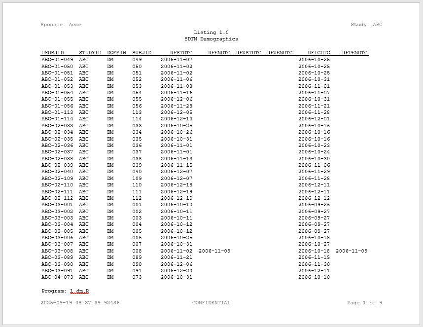
Generate a Listing
To generate the listing, we will need two files:
- A macro driver script
- A template listing program
Macro Driver Script
Here is the macro driver script:
#%%%%%%%%%%%%%%%%%%%%%%%%%%%%%%%%%%%#
#% Define Macro Variables
#%%%%%%%%%%%%%%%%%%%%%%%%%%%%%%%%%%%#
#%let sponsor_name <- Acme
#%let study_name <- ABC
#%let prog_name <- l_dm
#%let base_dir <- c:/packages/macro/tests/testthat/examples
#%let output_dir <- &base_dir./output
#%let data_dir <- &base_dir./data
#%let data_file <- dm.rda
#%let titles <- c("Listing 1.0", "SDTM Demographics")
#%let footnotes <- c("Program: &prog_name..R")

#%%%%%%%%%%%%%%%%%%%%%%%%%%%%%%%%%%%#
#% Pull in listing template code
#%%%%%%%%%%%%%%%%%%%%%%%%%%%%%%%%%%%#
#%include '&base_dir./templates/lst01.R'
As you can see, the macro driver is very simple. All it does is assign the necessary macro variables, and include the listing template.
Template Listing Program
Here is the template listing program:
#####################################################################
# Program Name: &prog_name.
# Study: &study_name.
#####################################################################

library(reporter)

# Output path
out_pth <- "&output_dir./&prog_name."

# Get listing data
load("&data_dir./&data_file.")

# Create table object
tbl <- create_table(dm) |>
  define(USUBJID, id_var = TRUE)

# Create report object
rpt <- create_report(out_pth, font = "Courier", output_type = "RTF") |>
  page_header("Sponsor: &sponsor_name.", "Study: &study_name.") |>
  titles(`&titles.`) |>
  add_content(tbl, align = "left") |>
  footnotes(`&footnotes.`) |>
  page_footer(Sys.time(), "CONFIDENTIAL", "Page [pg] of [tpg]")

# Write report to file
write_report(rpt)
Notice in the above code that there are several macro variables. They start with an ampersand (“&”) and sometimes end with a dot (“.”). These macro variables will be replaced with real values when the macro driver runs.
Also notice that the macro variables can be located anywhere in the program: in comments, in text strings, or in open code. The resolution routine will examine the entire program from top to bottom, replacing values as it goes.
How To Run
To run the macro, we will simply call msource() from the
command line. We will pass the name of the program to run and the
generated code file to output. Like this:
msource("./macro/Example1.R", "./macro/code/l_dm1.R")Generated Code
Upon execution, the generated code file will look like this:
#####################################################################
# Program Name: l_dm
# Study: ABC
#####################################################################

library(reporter)

# Output path
out_pth <- "c:/packages/macro/tests/testthat/examples/output/l_dm"

# Get listing data
load("c:/packages/macro/tests/testthat/examples/data/dm.rda")

# Create table object
tbl <- create_table(dm) |>
  define(USUBJID, id_var = TRUE)

# Create report object
rpt <- create_report(out_pth, font = "Courier", output_type = "RTF") |>
  page_header("Sponsor: Acme", "Study: ABC") |>
  titles(c("Listing 1.0", "SDTM Demographics")) |>
  add_content(tbl, align = "left") |>
  footnotes(c("Program: l_dm.R")) |>
  page_footer(Sys.time(), "CONFIDENTIAL", "Page [pg] of [tpg]")

# Write report to file
write_report(rpt)
Notice that all macro variables have been resolved, and the code is easily readable. The code actually looks like a human wrote it. Readability is a major advantage of generating code instead of writing a generalized program.
This technique gives you the best of all worlds: It is easy to build and maintain, allows a high degree of code reuse, provides flexible parameterization, and yet still produces simple, readable programs. These readable programs will be greatly appreciated by anyone who reviews your work.